How to: Reference: |
The Cox regression, also referred to as the proportional hazard model, is the most general of the regression models because it is not based on any assumptions concerning the nature or shape of the underlying survival distribution and the corresponding hazard function. The Cox regression predicts individual risk relative to the population.
The parametric survival regression, also referred to as the accelerated failure time model, assumes a particular distribution, such as Weibull, exponential, Gaussian, logistic, lognormal, and log-logistic. In RStat, the default distribution is set to Weibull. The parametric regression predicts the expected time to the event of interest.
What Is Survival Analysis?
A survival model is used to analyze time-to-event historical data and to generate estimates, referred to as survival curves, that show how the probability of the event occurring changes over time. In many life situations, as time progresses, certain events are more likely to occur. The survival models help decision makers to form better estimates than guessing about the expected timing of certain events. The estimates take into account the impact of other variables, referred to as independent, predictor variables or covariates, on the expected timing of the event to occur. A survival analysis can be used to determine not only the probability of failure of manufacturing equipment based on the hours of operations, but also to differentiate between different operating conditions. For example, if the probability changes if the machine is used outdoors versus indoors. For a detailed discussion on independent variables, see Building a Linear Regression Model.
Originally developed in the biomedical sciences to analyze time to death either of patients or of laboratory animals, survival analysis is now widely used in engineering, economics, finance, healthcare, marketing, and public policy.
How Does Survival Analysis Work?
Analogous to a linear regression analysis, a survival analysis typically examines the relationship of the survival variable (the time until the event) and the predictor variables (the covariates). The event of interest is frequently referred to as a hazard. The analysis specifies a linear-like function for the event called the hazard function. Below is the log hazard function, which is analogous to the linear regression function in Building a Linear Regression Model.
log hI(t) = α + β1x1 + β2x2 + βIxn
where:
Under this model, each covariate either increases or decreases the expected hazard, analogous to the predictor of linear regression. For more information on linear regression, see Building a Linear Regression Model.
There are several well known variations of the survival function, such as the multiplicative model or the proportional hazards model used in the Cox regression. While the math may differ, the conceptual understanding remains the same. Since the technical details of those functions are well documented in the statistical literature, we will omit them from the present discussion.
If survival analysis is so much like regression, why use a different modeling technique? Why not use linear regression?
Survival analysis methods are explicitly designed to deal with data about terminal events where some of the observations can experience the event and others may not. Such observations are called censored observations. For example, the target variable represents the time to a terminal event, and the duration of the study is limited in time. Therefore, some observations will not experience the event. Some equipment will fail during the time in which we monitor performance, but some will not.
There are two types of censoring, right and left censoring. Right censoring is most common and it occurs when the study expires or an individual or an item is removed from the study before the event occurs. For example, some individuals may still be alive at the end of a clinical trial, or may drop out of the study for various reasons other than death prior to the termination of the study. An observation is left-censored if its initial time at risk is unknown. This will occur if we do not know when a participant experienced for the first time the condition of interest. For example, when an individual contracted a disease.
The diagram below shows the distinct types of censoring.
Censoring complicates the estimation of the survival function. It requires different techniques than linear regression. Thus, in addition to the target variable, survival analysis requires a status variable that indicates for each observation whether the event has occurred or not and the censoring.
Practical Applications of Survival Analysis
Survival analysis is used for:
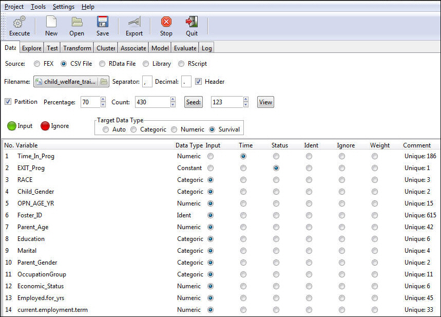
In this example, we are going to create a model for matching children with foster parents. We will use historical data that contains observations on the length of stay of children with foster parents. The predictor variables for the length of stay include child characteristics, such as age and gender, and foster parent characteristics, such as age and occupation.
The time variable has to be a continuous numeric variable representing time.
Your screen should look as below.
Survival is the only available method and Cox Proportional Hazards is set as the default choice.
The model output appears in the bottom window of the Model tab, as shown in the following image.
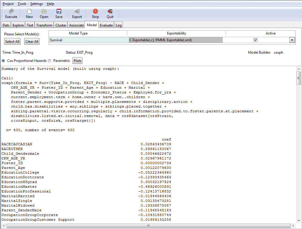
This section describes the Cox Proportional Hazard regression output.
Summary of the Cox regression model. This is the title of the summary provided for the model.
Summary of the Survival model (built using coxph)
R Function Call.
coxph(formula = Surv(TIME_IN_PROG, EXIT_PROG) ~ RACE + CHILD_GENDER +
    OPN_AGE_YR + PARENT_AGE + EDUCATION + MARITAL + PARENT_GENDER +
    OCCUPATIONGROUP + ECONOMIC_STATUS + EMPLOYED_FOR_YRS + CURRENT_EMPLOYMENT_TERM,
    data = crs$dataset[, ])
where:
Is the library in R that is used to construct the hazard function.
The formula lists the survival target and status variable (Surv(time, status)) and the covariates (age, education, marital, and so on). The data section shows which columns from the data sets are used in the model. In this case, we use all the columns from the data set.
Indicates the number of observations used for training the model.
Coefficients are shown in the following image.
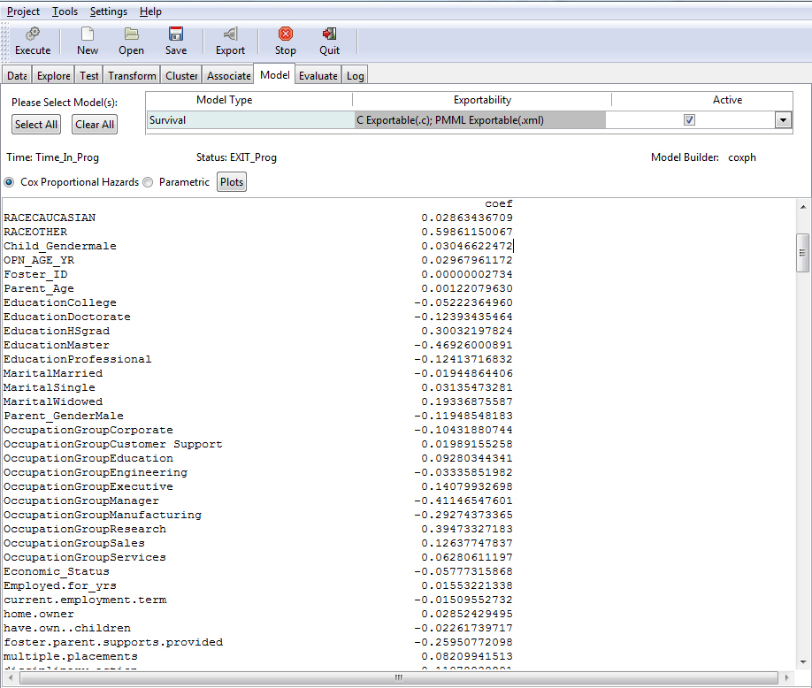
This part of the output shows the coefficients, their standard errors, the z-statistic, and associated Pr(z)-values.
Note: To view additional data regarding the coefficients, use the down arrow to scroll through the output.
The closer the P values are to zero, the more significant the coefficient is. The z statistics records the ratio of each regression coefficient to its standard error. The Z statistics are analogous to the F in the linear regression, see Output From Linear Regression.
The second column displays the exponentiated coefficient. The exponent of the estimated coefficient is the odds ratio (hazard ratio) which can be used to estimate directly the percent of risk that each coefficient contributes to the overall hazard. For example, holding all other covariates constant, a child gender=female reduces the hazard of a child leaving the program by a factor of e^(CHILD_GENDERFemale) = 0.943859, or it will reduce the risk by 1- 0.943859 = 0.056, or by 5.6%.
The significance codes indicate the level of significance of each coefficient. (See Output From Linear Regression for more information on significance codes.) For example, OCCUPATIONGROUPSales is significant as indicated by the "*". Its significance can also be inferred from the small Pr(z) value of 0.0492.
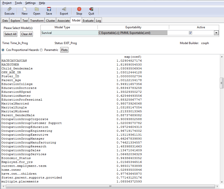
The following image shows the continued output for the coefficients table. It shows the exponentiated coefficient and the 95% confidence interval (upper and lower bound) for the exponentiated coefficient.
The exp(--coef) is the inverted hazard ratio. The exp(coef) shows the hazard ratio between female versus male. The inverted hazard ratio shows the male versus female odds ratio.
Note: The data for exp(coef) and exp(-coef) are in different sections. To view each, use the down arrow to scroll down through the output.
The image below shows the model diagnostics statistics.
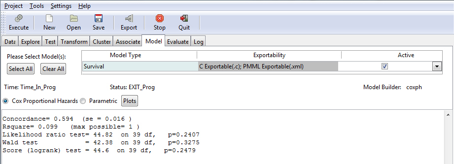
Rsquare. Is a measure of the proportion of variability explained by the regression. It is a number between zero and one, and a value close to zero suggests a poor linear regression model. (See Output From Linear Regression for more information.) Although the generalized R-squared is commonly recommended for the Cox model, it must be noted that it is highly sensitive to the proportion of censored values. The expected value of R-squared decreases substantially as a function of the percent censored observations. Average Rsquare values can decrease by 20% or more with heavy censoring.
Likelihood ratio tests, the Wald test, and the Score tests. All three tests are global tests evaluating the hypothesis that the coefficient estimates are different from zero, or in other words that they contribute to the prediction of the hazard. The closer the test result is to zero, the more likely it is that the coefficients are different from zero and thus do contribute to the prediction. The degrees of freedom (df) are equal to the number of parameters in the model minus the number of parameters of a reduced model, for example a model without the coefficients that are equal to zero. Usually the three tests give very similar results. Sometimes the Wald statistics may be different from the Likelihood ratio test for various reasons, and there are many reasons given in the statistical literature why the likelihood ratio test should be used instead of the Wald when the two tests disagree. Those theoretical discussions fall outside of the scope of the present manual. The score test is more useful when the survival distributions of two samples are compared. For example, in clinical trials the score test is used to establish the efficacy of a new treatment compared to a control treatment when the measurement is the time-to-event (such as the time from initial treatment to a heart attack).
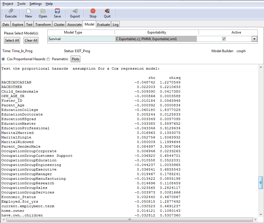
The following image shows the tests for proportional hazard assumptions. The proportional hazard regression assumes that for any two groups or strata the survival curves are proportionate over time. The condition implies that the covariates multiply the hazard. The output is a matrix with one row for each variable and a last row for the global test. The columns of the matrix contain the correlation coefficient between transformed survival time and the scaled Schoenfeld residuals (see How to Generate Survival Analysis Plots), a chi-square, and the two-sided p-value. For the global test there is no appropriate correlation, so an NA is entered into the matrix as a placeholder. The closer the p-value is to zero, the stronger the evidence of the existence of a non-proportional hazard, a hazard that varies over time and thus impacts the effectiveness of the prediction. The presence of a non-proportional hazard requires some corrective actions, many of which are documented in the statistical literature but are outside of the scope of this manual.
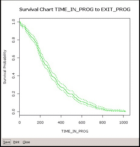
To generate a plot, click the Plot button.
Two charts are generated, a Survival chart and a Scaled Schoenfeld Residuals chart. The Plot option is available only for a Cox regression.
The Survival chart plots the probability of survival (Y) against Time (X). The two dashed line represent the 95% confidence interval.
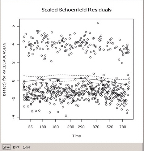
Schoenfeld residuals are used to test the assumption of proportional hazards. Schoenfeld residuals "can essentially be thought of as the observed minus the expected values of the covariates at each failure time" (Steffensmeier & Jones, 2004: 121). There is a Schoenfeld residual for each subject for each covariate. The image below shows the SSR for the RACECAUCASIAN coefficient. The plot of Schoenfeld residuals against time for any covariate should not show a pattern of changing residuals for that covariate. If there is a pattern, that covariate is time-dependent. As a rule of thumb, a non-zero slope is an indication of a violation of the proportional hazard assumption. The dotted lines outline the 95% confidence interval.
| WebFOCUS |