How to: Reference: |
What Is Regression Analysis?
Regression analysis is the method of using observations (data records) to quantify the relationship between a target variable (a field in the record set), also referred to as a dependent variable, and a set of independent variables, also referred to as a covariate. For example, regression analysis can be used to determine whether the dollar value of grocery shopping baskets (the target variable) is different for male and female shoppers (gender being the independent variable). The regression equation estimates a coefficient for each gender that corresponds to the difference in value.
The value of quantifying the relationship between a dependent variable and a set of independent variables is that the contribution of each independent variable to the value of the dependent variable becomes known. Once this is known, you need to know only the values of the independent variables in order to be able to make predictions about the value of the dependent variable. For example, when the coefficients for male and female shoppers are known, you can make precise revenue estimates for different distributions of shoppers. Specifically, you can predict the revenues for 80/20 females/males versus 60/40 females/males.
The goal of regression analysis is to generate the line that best fits the observations (the recorded data). The rationale for this is that the observations vary and thus will never fit precisely on a line. However, the best fitted line for the data leaves the least amount of unexplained variation, such as the dispersion of observed points around the line. Stated differently, a relationship that explains 90% of the variation in the observations is better than one that explains 75%. Conversely, a relationship with a better fit has a better predictive power.
How Does Linear Regression Work?
To illustrate how linear regression works, examine the relationship between the prices of vintage wines and the number of years since vintage. Each year, many vintage wine buyers gather in France and buy wines that will mature in 10 years. There are many stories and speculations on how the buyers determine the future prices of wine. Is the wine going to be good 10 years from now, and how much would it be worth? Imagine an application that could assist buyers in making those decisions by forecasting the expected future value of the wines. This is exactly what economists have done. They have collected data and created a regression model that estimates this future price. The current explanation of the regression is based on this model.
The provided sample data set contains 60 observations of prices for vintage wines that were sold at a wine auction. There are two columns, one for the price of each wine and another for the number of years since vintage. The data set, referred to as the training data set, is used to estimate the parameters in the equation.
The estimated equation can be used to predict wine prices when the year since vintage is known. In other words, it can be applied to another data set, referred to as the test data set, which contains only vintage years. Prices are derived by applying the equation to the vintage years in the training data set.
The following formula describes the linear relationship between price and years:
y = β0 + β1 x + error
The following image visually examines the nature of the relationship by plotting Y and X on a scatter plot with the trend line.
The following regression equation shows estimated parameters for the trend line:
y = -533 + 55 * xTo predict the price for a 15-year-old vintage wine, substitute x=15:
y = -533 + 55 * 15
y = -533 + 825
y = 292
How Does Multiple Linear Regression Work?
A simple linear equation rarely explains much of the variation in the data and for that reason, can be a poor predictor. In the case of vintage wine, time since vintage provides very little explanation for the prices of wines. The regression equation described in the simple linear regression section will poorly predict the future prices of vintage wines. Multiple linear regression enables you to add additional variables to improve the predictive power of the regression equation. On a very intuitive level, the producer of the wine matters. Thus, including the chateau as another independent variable is likely to increase the predictive power of the equation.
The following equation shows a multiple linear regression equation. The equation is conceptually similar to the simple regression equation, except for parameters β2 through βn, which represent the additional independent variables.
y = β0 + β1x1 + β2x2 + ... + βnxn + error
The independent variables in the vintage wine data set are:
The regression equation estimates a single parameter for the numeric variables and separate parameters for each unique value in the categorical variable. For example, there are six chateaus in the data set, and five coefficients. One chateau is used as a base against which all other chateaus are compared, and thus, no coefficient will be estimated for it. In other words, if prices have to be predicted for the reference chateau, 0 is entered in the equation.
The equation with the estimated parameters is:
Price = - 4744 + 1.03 * WR + 295.84 * T - 2.09 * HR + 8.06 * TSV + Chateau
The coefficients for each chateau are given in the output, as shown in the following image.
                         Estimate Std. Error t value   Pr(>|t|)
(Intercept)            -4743.7592  1027.7697  -4.616 0.00002762 ***
WRAIN                      1.0287     0.2513   4.093   0.000155 ***
DEGREES_IN_C             295.8356    58.8231   5.029 0.00000672 ***
HRAIN                     -2.0854     0.3686  -5.658 0.00000074 ***
TIME_SINCE_VINTAGE         8.0633    10.9301   0.738   0.464133
CHATEAUCos d'Estournel  -280.2000    99.3542  -2.820   0.006863 **
CHATEAULafite              7.8000    99.3542   0.079   0.937738
CHATEAULatour            177.9000    99.3542   1.791   0.079418 .
CHATEAUMontrose         -320.8000    99.3542  -3.229   0.002198 **
CHATEAUPichon Lalande   -228.4000    99.3542  -2.299   0.025730 *
---
Tip: The image below shows how the estimated parameter values are used as the coefficient values in the regression equation.
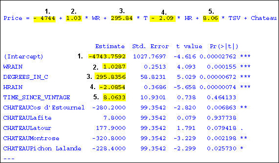
Note: Cheval Blanc is the reference chateau with a coefficient of 0. Therefore, it is not listed in the output. However, when scoring data, the predicted prices for the Cheval Blanc will be in the scoring output. For more information about the output, see Output From Linear Regression.
Vintage wine prices can be predicted by substituting the values for the independent variables, as in the simple regression equation used earlier.
A scoring application automatically generates the predicted prices, either for a single record or for a batch of records.
Practical Applications of Regression Analysis
Regression analysis is used for:
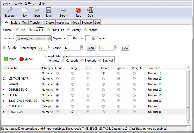
Note: The following example creates a multiple linear regression, using the wine_train data source, and targets PRICE_1991.
The status bar confirms your data settings, as shown in the following image.
Note: Other available regression models are Generalized (Gaussian Regression model) and Poisson Regression models. Both models are built using Regression Generalized (glm).
The model data output appears in the bottom window of the Model tab, as shown in the following image.
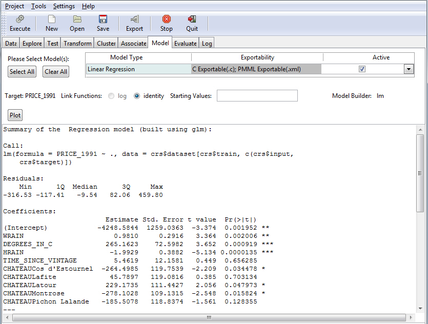
For details about the regression output, see Output From Linear Regression.
This section describes the linear regression output. Note that output may vary slightly due to sampling.
Summary of the Regression model (built using lm):
lm(formula = Price_1991 ~ ., data = crs$dataset[, c(3:8)])
 Min       1Q   Median       3Q      Max
-404.62 -135.97   -9.47  95.58  4484.79
Coefficients:
Coefficients:
                         Estimate Std. Error t value Pr(>|t|)
(Intercept)            -5191.3914  1405.3794  -3.694 0.000820 ***
WRAIN                      0.9171     0.3502   2.619 0.013373 *
Degrees_in_C             329.9655    83.0036   3.975 0.000375 ***
HRAIN                     -1.8965     0.4753  -3.990 0.000360 ***
Time_Since_Vintage         7.3211    13.6187   0.538 0.594587
ChateauCos d'Estournel  -336.9234   130.7021  -2.578 0.014753 *
ChateauLafite            -70.7367   128.0801  -0.552 0.584590
ChateauLatour            -27.4525   136.1005  -0.202 0.841422
ChateauMontrose         -365.6623   140.1642  -2.609 0.013698 *
ChateauPichon Lalande   -283.3606   120.9652  -2.342 0.025538 *
---Signif. codes:
0 '***' 0.001 '**' 0.01 '*' 0.05 '.' 0.1 ' ' 1
The significance codes indicate how certain we can be that the coefficient has an impact on the dependent variable. For example, a significance level of 0.01 indicates that there is less than a 0.1% chance that the coefficient might be equal to 0 and thus be insignificant. Stated differently, we can be 99.9% sure that it is significant. The significance codes (shown by asterisks) are intended for quickly ranking the significance of each variable.
Residual standard error: 237.4 on 37 degrees of freedom.
Multiple R-squared: 0.7958
Adjusted R-squared: 0.7384
F-statistic: 13.86 on 9 and 32 DF, p-value: 0.000000009629.
For example, 50 = 60 - 1- 9.
The F-value is the Mean Square Regression divided by the Mean Square Residual. It is calculated on 9 Df for the coefficients and 50 Df for the residuals.
The P-value associated with this F-value is very small (5.596e-15). The P-value is a measure of how confident you can be that the independent variables reliably predict the dependent variable. P stands for probability and is usually interpreted as the probability that test data does not represent accurately the population from which it is drawn. If the P-value is 0.10, there is a 10% probability that the calculation for the test data is not true for the population. Conversely, you can be 90% certain that the results of the test data are true of the population.
For example, if the P-value were greater than 0.05, the group of independent variables does not show a statistically significant relationship with the dependent variable, or that the group of independent variables does not reliably predict the dependent variable. Note that this is an overall significance test assessing whether the group of independent variables when used together reliably predict the dependent variable, and does not address the ability of any of the particular independent variables to predict the dependent variable. The ability of each individual independent variable to predict the dependent variable is addressed in the coefficients table. (See P-values for the regression coefficients.)
The following image shows the Model tab with the ANOVA table for the regression output. The ANOVA table provides statistics on each variable used in the regression equation.
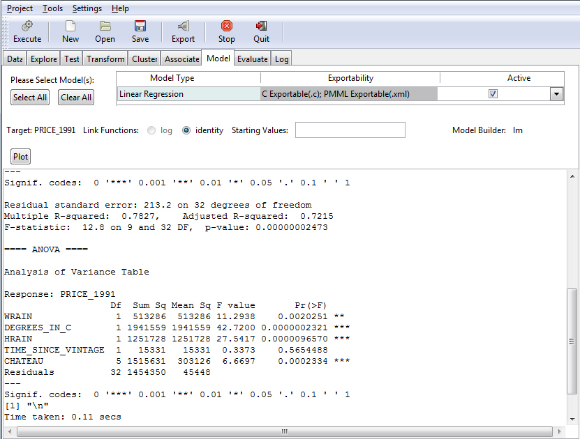
                   Df  Sum Sq Mean Sq F value    Pr(>F)
WRAIN               1 2208522 2208522 44.7465 1.838e-08 ***
Degrees_in_C        1 4462834 4462834 90.4208 8.508e-13 ***
HRAIN               1 1702437 1702437 34.4928 3.445e-07 ***
Time_Since_Vintage  1   26861   26861  0.5442    0.4641
Chateau             5 1962422  392484  7.9521 1.422e-05 ***
Residuals          50 2467813   49356
---
0 '***' 0.001 '**' 0.01 '*' 0.05 '.' 0.1 ' ' 1
The significance codes indicate how certain we can be that the coefficient has an impact on the dependent variable. For example, a significance level of 0.001, indicates that there is less than a 0.1% chance that the coefficient might be equal to 0 and thus be insignificant. Stated differently, we can be 99% sure that it is significant. The significance codes (shown by asterisks) are intended for quickly ranking the significance of each variable.
The time taken to generate the parameter estimates.
| WebFOCUS |