In this section: How to: |
Using RStat, you can define and execute various models against a selected database.
Note:
- Depending on your data, certain model types may be disabled.
- The Ada Boost option is selected by default.
- You can click Select All to select all relevant models, or select one or multiple models to perform a simultaneous analysis. To view the output of other models that were selected for simultaneous execution, click the model type within the Model Type table.
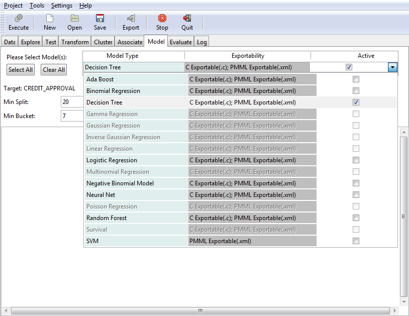
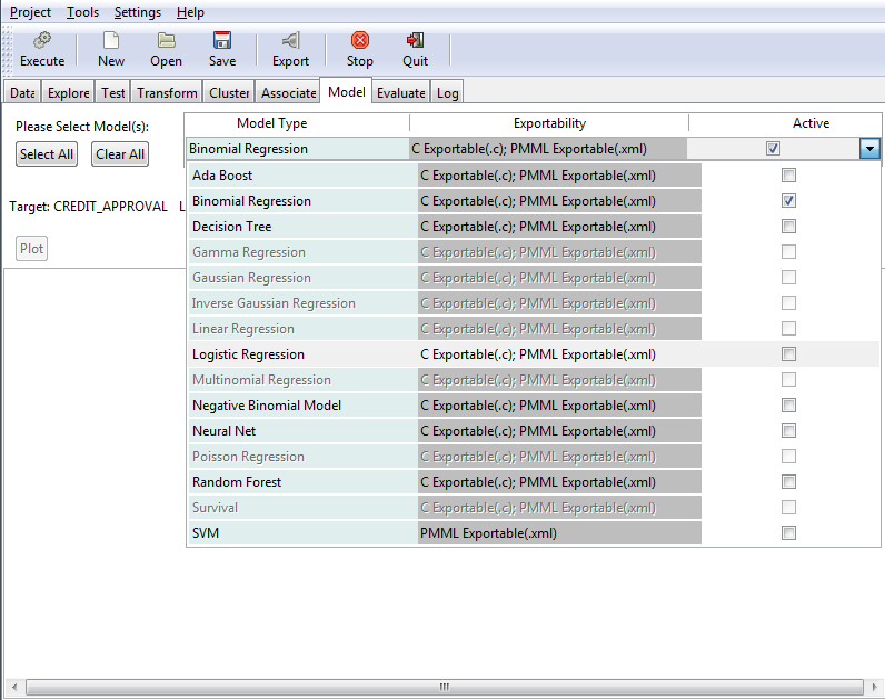
The supported model types and their exportability are listed in the following table.
|
Model Type |
Exportability |
|---|---|
|
Ada Boost |
C Exportable(.c);PMML Exportable(.xml) |
|
Binomial Regression |
C Exportable(.c);PMML Exportable(.xml) |
|
Decision Tree |
C Exportable(.c);PMML Exportable(.xml) |
|
Gamma Regression |
C Exportable(.c);PMML Exportable(.xml) |
|
Gaussian Regression |
C Exportable(.c);PMML Exportable(.xml) |
|
Inverse Gaussian Regression |
C Exportable(.c);PMML Exportable(.xml) |
|
Linear Regression |
C Exportable(.c);PMML Exportable(.xml) |
|
Logistic Regression |
C Exportable(.c);PMML Exportable(.xml) |
|
Multinomial Regression |
C Exportable(.c);PMML Exportable(.xml) |
|
Negative Binomial |
C Exportable(.c);PMML Exportable(.xml) |
|
Neural Net |
C Exportable(.c);PMML Exportable(.xml) |
|
Poisson Regression |
C Exportable(.c);PMML Exportable(.xml) |
|
Random Forest |
C Exportable(.c);PMML Exportable(.xml) |
|
Survival |
C Exportable(.c);PMML Exportable(.xml) |
|
SVM |
PMML Exportable(.xml) |
The following procedure provides basic guidance for executing a model type option.
- Open RStat.
- Click the folder adjacent to the Filename field and select a data set.
- Click Execute to load the data.
- Click the Model tab.
- Select a model type.
- Select or populate fields based on the model type that you select. For more information, refer to each of the model options discussed in this section.
-
Click Execute to
view the model based on your selections.
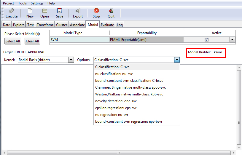
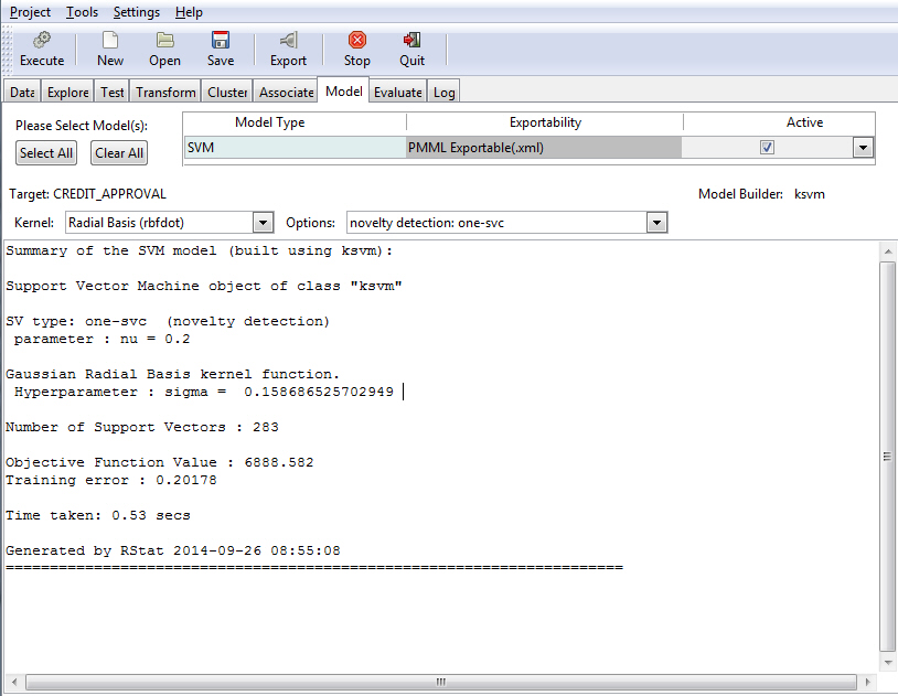
For example, the following image illustrates the results of modeling using SVM with the default Kernel value selected (Radial Basis (rbfdot)). The novelty detection: one-svc option was selected.
The following sections present key functionality for each of the different model types.
The Ada Boost model uses the ada, which is the underlying algorithm (model builder). Boosting builds multiple, but generally simple, models. The models might be decision trees that have just one split. These are commonly referred to as decision stumps.
Note:
- The Ada Boost model returns class and probability.
- Ada Boost is for non-regression binary trees.
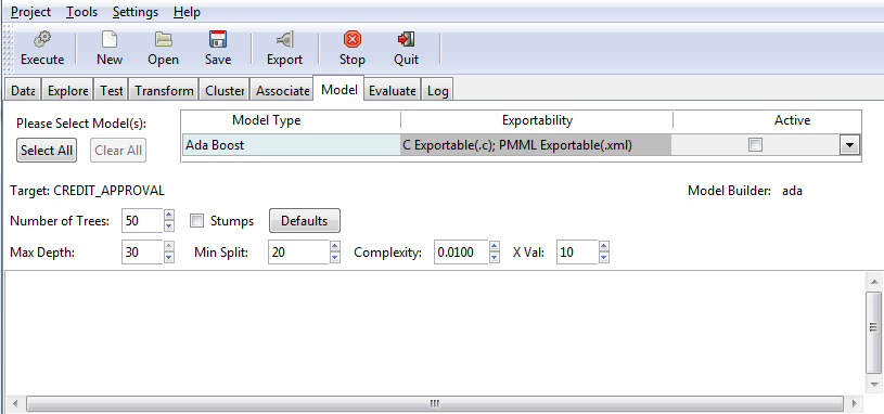
The Boost model allows you to specify the number of trees, in addition to other criteria, as shown in the following image.
The following table lists and describes the fields that are used to adjust the Boost model.
|
Field Name |
Description |
|---|---|
|
Number of Trees |
The number of trees to build. Note: In order to ensure that every input row is predicted at least a few times, this value should not be set to a number that is too low. The default value is 50. |
|
Max Depth |
Allows you to set the maximum depth of any node of the final tree. The root node is counted as depth 0. The default value is 30. Note: Values greater than 30 will generate invalid results on 32-bit machines. |
|
Stumps |
If the Stumps check box is selected, you can build stumps using the Boost model. If the Stumps check box is not selected, the results in the default values are deactivated. |
|
Min Split |
The minimum number of entities that must exist in a data set at any node for a split of that node to be attempted. The default value is 20. |
|
Complexity |
Also known as the complexity parameter (cp), this value allows you to control the size of the decision tree and select the optimal size tree. If the cost of adding another variable to the decision tree from the current node is above the value of the cp, then tree building does not continue. The default value is 0.0100. Note: The main role of this parameter is to save computing time by pruning unnecessary splits. |
|
X Val |
Refers to the number of cross-validation errors allowed. The default value is 10. |
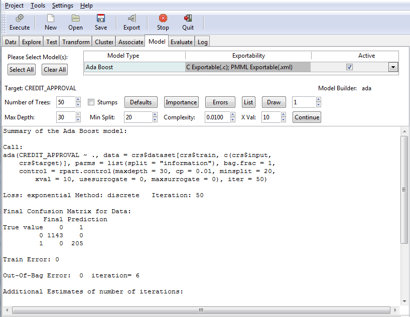
Once you have defined your model criteria, you must click the Execute button to review the results, as shown in the following image.
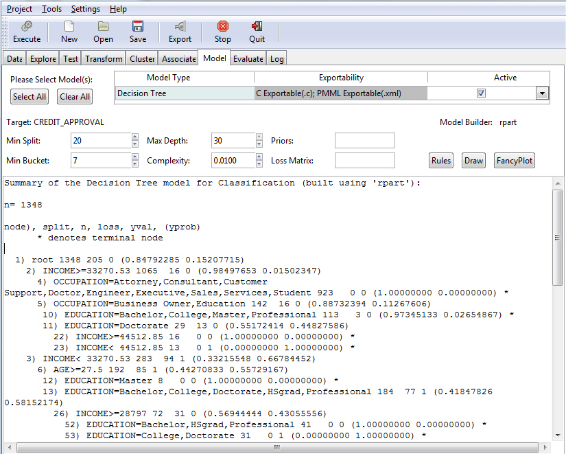
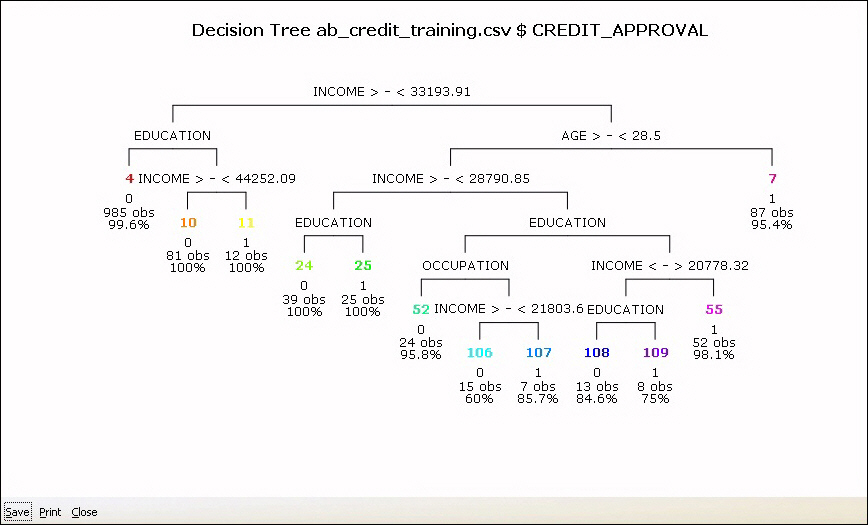
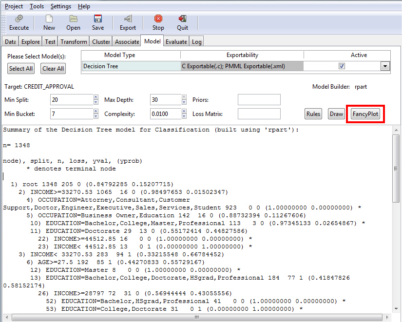
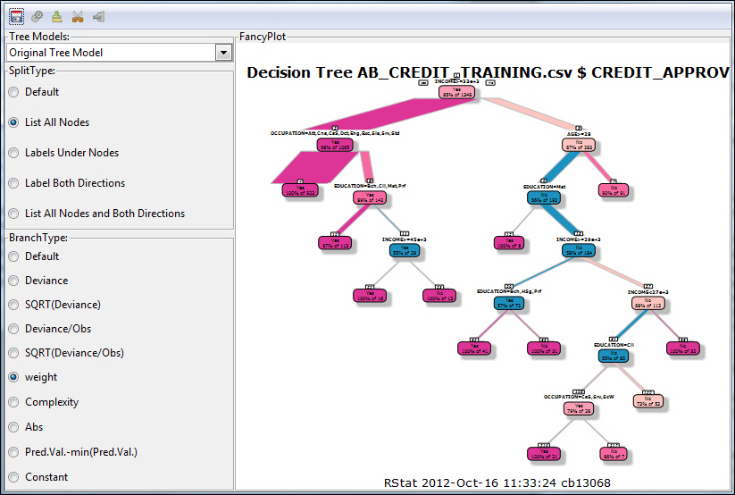
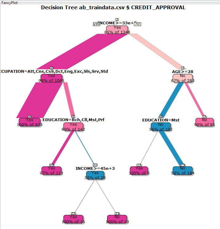
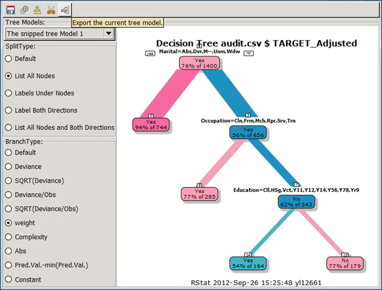
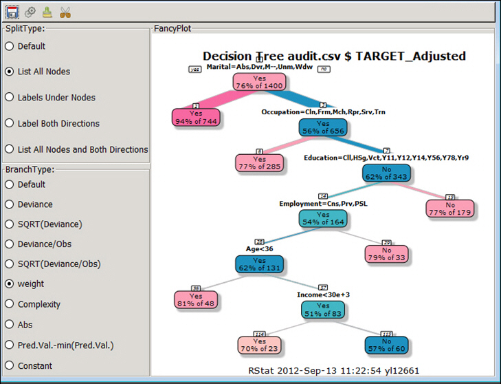
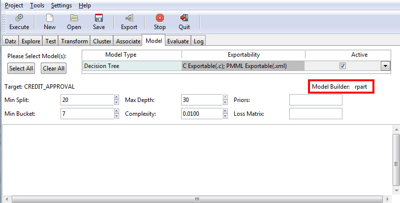
The Decision Tree option is used to generate a decision tree, which is the prototypical data mining technique. It is widely used because of its ease of interpretation. The Decision Tree model uses an underlying algorithm (model builder) of rpart, as shown in the following image.
The following table lists and describes the fields that are used to adjust a Decision Tree model.
|
Field Name |
Description |
|---|---|
|
Min Split |
The minimum number of entities that must exist in a data set at any node for a split of that node to be attempted. The default value is 20. |
|
Min Bucket |
The minimum number of entities allowed in any leaf node of the decision tree. The default value is one third of the min split. |
|
Max Depth |
Allows you to set the maximum depth of any node of the final tree. The root node is counted as depth 0. The default value is 30. Note: Values greater than 30 will generate invalid results on 32-bit machines. |
|
Complexity |
Also known as the complexity parameter (cp), this value allows you to control the size of the decision tree and select the optimal size tree. If the cost of adding another variable to the decision tree from the current node is above the value of the cp, then tree building does not continue. The default value is 0.0100. Note: The main role of this parameter is to save computing time by pruning unnecessary splits. |
|
Priors |
Allows you to set the prior probabilities for each class. |
|
Loss Matrix |
Allows you to weight the outcome classes differently. |
Once you have specified your model criteria, you must click the Execute button to view the result. Since Tree was selected, the Summary of the Decision Tree model displays, as shown in the following image.
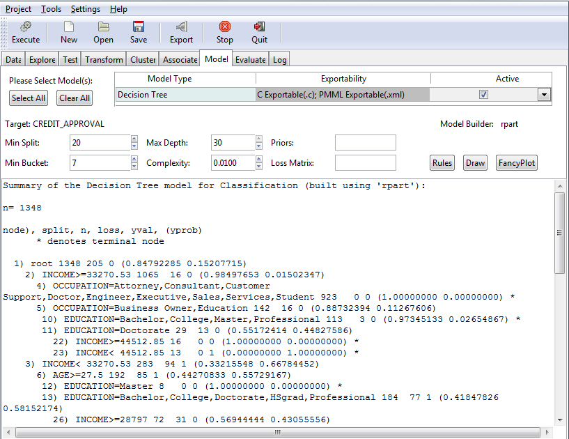
Note: The default values for all fields were used to create this example.
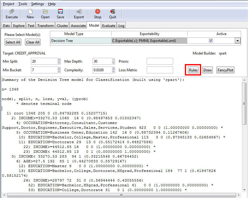
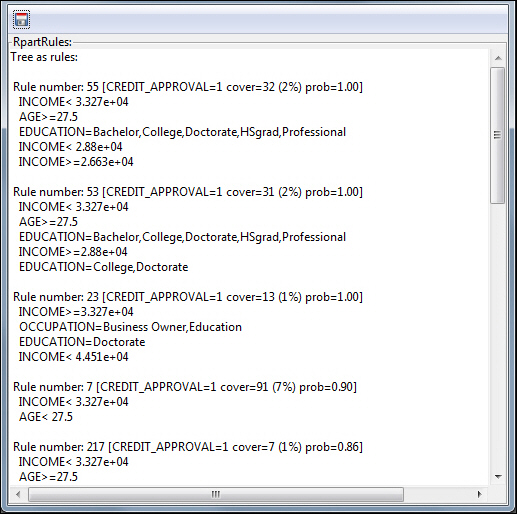
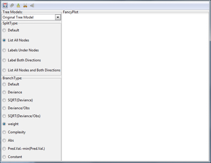
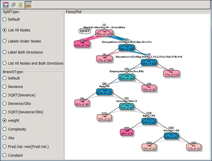
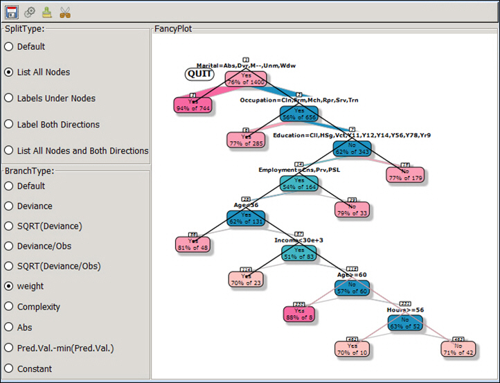
You can view the summary or access other features of the application, including Rules, Draw, and FancyPlots. For more information, see:
Regression is a traditional approach to modeling. The model builder glm (logit) is used by the Regression model. Logistic regression (using the binomial family) is used to model binary outcomes. Linear regression is used to model a linear numeric outcome. For predicting where the outcome is a count, the Poisson family is used. Generalized Regression is generalization of standard linear regression, allowing for response variables that fall outside of a normal distribution. Multinomial regression generalizes logistic regression, in that it allows more than two discrete outcomes. For more information, see Building a Logistic Model and Building a Linear Regression Model.
RStat supports regression and advanced regression, as shown in the following image.
The following techniques related to regression can be performed:
- Binomial. Distribution is binomial distribution, which is a discrete probability distribution of the number of successes in a sequence of a variable number (n) of dependent Yes or No experiments. The LinkFunction could be either logit, probit, or cauchit.
- Gamma. The error distribution is Gamma distribution. The LinkFunction could be inverse, identity, or log.
- Gaussian. The error distribution is normally distributed. The response method is dependent on the LinkFunction. The LinkFunction can be identity, log, or inverse.
- Inverse Gaussian. The error distribution is Gamma distribution. The LinkFunction could be inverse, identity, log, or 1/mu^2.
- Linear. The error distribution is normally distributed. The response variable is linear in relation to the predictive model.
- Logistic. Usually referred to as binomial or binary logistic regression, this is used to predict two possible types of outcome (YES or NO).
- Multinomial. Referred as multinomial logistic regression, this is used to predict three or more possible types of outcome.
- Negative Binomial. The error distribution is negative binomial distribution, which is a discrete distribution of the number of successes in a sequence of Bernoulli trials before a specified number of failures occur.
- Poisson. The error distribution or response variable distribution is Poisson distribution. Poisson regression is used to model and predict in cases where count data and contingency tables are used.
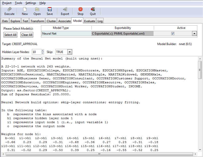
Neural Network (Neural Net) is an older approach to modeling. The Neural Net model uses a structure that resembles the neural network of a human being. When applied to modeling, the concept is to build a network of neurons that are connected by synapses. Rather than generate electrical signals, however, the network propagates numbers.
When using the Neural Net model, you can include or exclude the interval of networks from your model. The interval of networks is used to define and describe the relationships within your model. Display of these intervals is accomplished using the Skip field. When set to True (default), the interval of networks displays. If the Skip field is set to False, the interval of networks does not display.
The default value of True is shown in the following image.
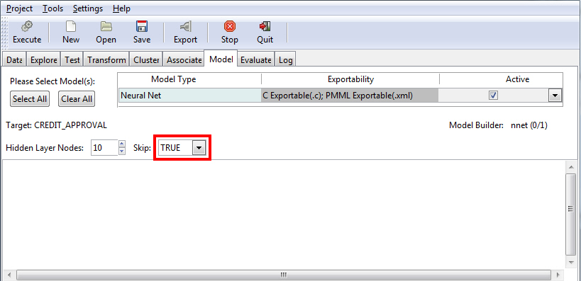
The following table lists the options that are available on the Neural Net model screen.
|
Field Name |
Description |
|---|---|
|
Hidden Layer Nodes |
The number of hidden layer nodes to display. The default is 10. |
|
Skip |
Set to a value of TRUE by default, this field switches between the input and output of skip-layer connections, depending on your selection. |
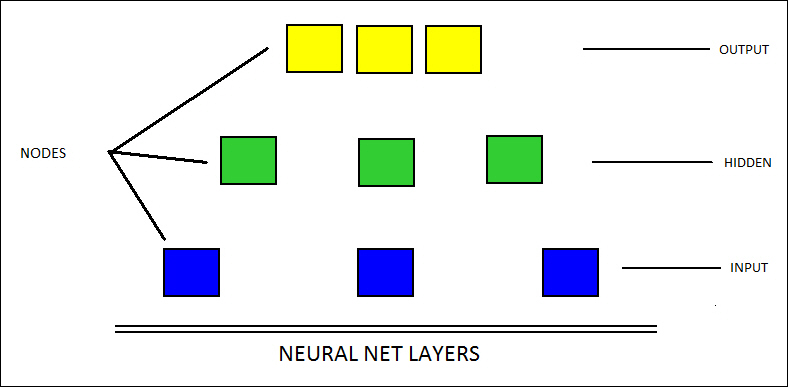
In the following diagram, the relationships between the different layers of a neural record are illustrated. The bottom portion represents the input layer, the middle nodes form the hidden layer, and the top components constitute the output layer.
Note: The number of nodes varies in different applications. In addition, you must have a data set selected and loaded in order to use this functionality.
The following example shows the results of a Neural Net model with the Skip field set to True. Accordingly, RStat displays the interval of networks.
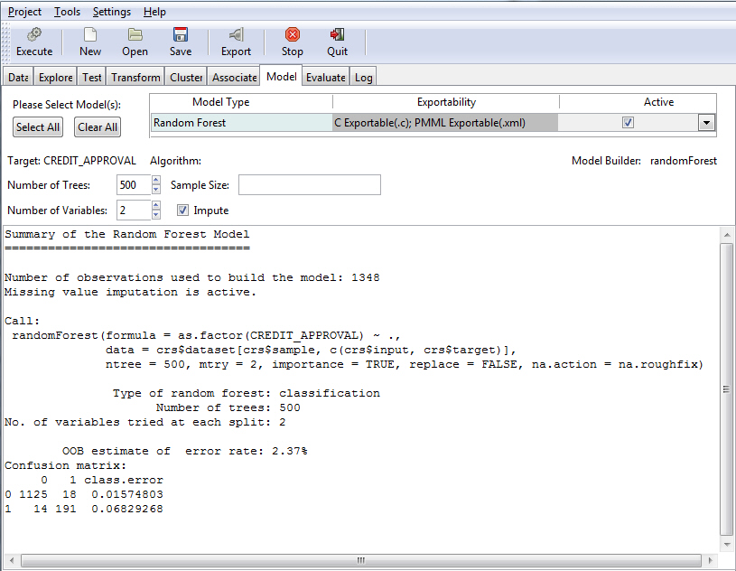
The Random Forest uses an underlying algorithm (randomForest), which builds multiple decision trees from different samples of the data set. While building each tree, random subsets of the available variables are considered for splitting the data at each node of the tree.
Note:
- When using the C export with the Random Forest model, class and regression(numeric values) are returned.
- Random Forest trees can be binary and k-ary(k>2).
You can specify a number of trees (the default is 500) and a number of variables (the default is 4), as shown in the following image.
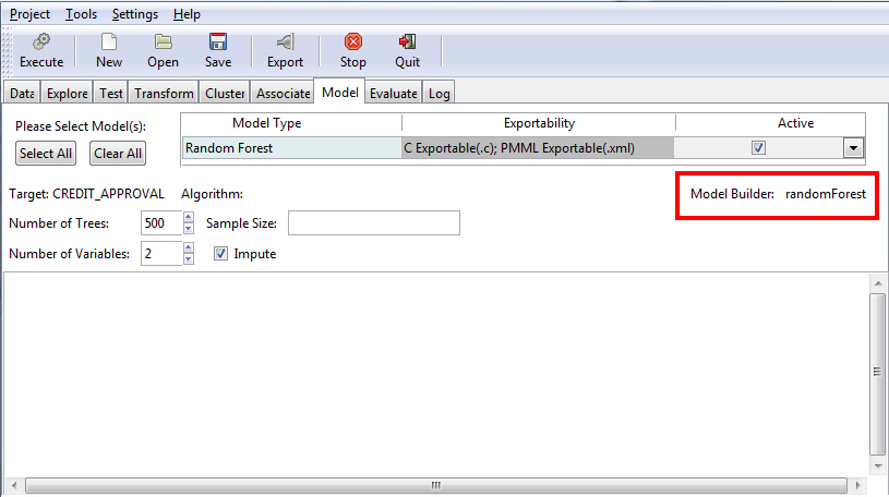
The following table lists and describes the fields that are used to adjust the Random Forest model.
|
Field Name |
Description |
|---|---|
|
Number of Trees |
The number of trees to build. Note: In order to ensure that every input row gets predicted at least a few times, this value should not be set to a number that is too low. The default value is 500. |
|
Number of Variables |
This is the number of variables to be considered at any time in deciding how to partition the data set. Each split produces a number of variables which are randomly sampled as candidates. |
|
Sample Size |
Size(s) of a sample to draw. |
|
Impute |
This applies to missing variables. If this check box is selected, the variables are transferred by replacing any NA values with one of the following (depending on the current selection):
|
Once you have indicated your criteria, you must click the Execute button to see the results, as shown in the following image.
The Survival Model is used to model time-to-event data. When using this option, you can select Cox Proportional Hazards (coxph) or Parametric (survreg) to perform your Survival Analysis, as shown in the following image. For more information on the Survival model, see Building a Survival Model.
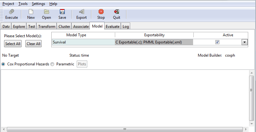
The following table lists and describes the fields that are used to adjust a Survival model.
|
Field Name |
Description |
|---|---|
|
Time |
The variable that you selected (time) on the Data tab. |
|
Status |
The variable that you selected (status) on the Data tab. |
|
Model Builder |
The name of the model builder (coxph or survreg) related to the selection you made: Cox Proportional Hazards or Parametric. |
|
Cox Proportional Hazards |
A general regression model that predicts individual risk relative to the population. |
|
Parametric |
Also known as the accelerated failure time model, this regression model predicts the expected time to the event of interest. |
|
Survival |
This option enables you to view the results of the Cox Proportional Hazards model. For more information, see Building a Survival Model. |
|
Residuals |
This button enables the testing of the assumption of proportional hazards. |