You can calculate trends in numeric data and predict
values beyond the range of those stored in the data source by using
the Forecast feature.
The calculations you can make to identify
trends and forecast values are:
xUsing a Simple Moving Average
A simple moving average is a series of arithmetic means
calculated with a specified number of values from a field. Each
new mean in the series is calculated by dropping the first value used
in the prior calculation, and adding the next data value to the
calculation.
Simple moving averages are sometimes used to analyze trends in
stock prices over time. In this scenario, the average is calculated
using a specified number of periods of stock prices. A disadvantage
to this indicator is that because it drops the oldest values from
the calculation as it moves on, it loses its memory over time. Also,
mean values are distorted by extreme highs and lows, since this
method gives equal weight to each point.
Predicted values beyond the range of the data values are calculated
using a moving average that treats the calculated trend values as
new data points.
The first complete moving average occurs at the nth data
point because the calculation requires n values. This is
called the lag. The moving average values for the lag rows are calculated
as follows: the first value in the moving average column is equal
to the first data value, the second value in the moving average
column is the average of the first two data values, and so on until
the nth row, at which point there are enough values to
calculate the moving average with the number of values specified.
x
Procedure: How to Calculate a Simple Moving Average
-
With
the By or Across field you want to use for your calculations, click Forecast.
The Forecast dialog box opens.
-
If you
want to change the name of the output field that displays the Forecasted
values, edit the default name that exists in the Field Name field.
-
Click Moving
Average from the Step 1: Choose a Method drop-down list.
-
Select
an input measure field from the Step 2: Choose a Measure drop-down
list.
If you select the same field as the By or Across field,
this field will not appear in the output even if it is included
in a display command.
-
Select
the increment number to count each instance of the By or Across
field from the Step 3: Choose The Interval menu.
-
Select
the number of predictions to be calculated for the Forecast field
from the Step 4: Choose Number of Predictions menu.
-
Select
the number of values to average from the Step 5: Choose Number Of
Values to Average menu.
-
Optionally,
change the default field format by clicking the Change
Format button and selecting a different format from
the Format dialog box.
-
Click OK.
x
Reference: Forecast Dialog Box - Moving Average
The
Forecast dialog box is shown in the following image.
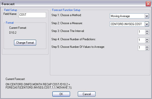
The
Forecast dialog box contains the following fields or options.
Field Setup
-
Field Name
- Is the Forecast field name.
-
Current Format
- Displays the format of the Forecast.
-
Change Format
- Opens the Format dialog box.
-
Forecast Function Setup
-
Step 1: Choose a Method
- Is the Forecast method to use to predict values. The options
are:
Double Exponential Average. Accounts for the tendency
of data to either increase or decrease over time without repeating.
Exponential Average. Calculates
a weighted average between the previously calculated value of the
average and the next data point.
Linear Regression. Derives
the coefficients of a straight line that best fits the data points
and uses this linear equation to estimate values.
Moving Average. Calculates
a series of arithmetic means using a specified number of values
from a field.
Multivariate Regression. Predicts two
or more dependent variables using one independent variable.
Triple Exponential Average. Accounts
for the tendency of data to repeat itself in intervals over time.
-
Step 2: Choose a Measure
- Is the field to be used to calculate the Forecast field.
-
Step 3: Choose The Interval
- Is the increment by which to count instances of the By or Across
field.
-
Step 4: Choose Number of Predictions
- Is the number of predictions to be calculated.
-
Step 5: Choose Number Of Values to Average
- Is the number of values to use to calculate the average used
to predict values.
-
Current Forecast
- Displays the code created by the Forecast dialog box.
Example: Calculating a Simple Moving Average
Create a new procedure, open with Report
Painter, and open the centord.mas file.
- Select Report at
the top of the Report Painter window, then select Define from
the drop-down list.
The Define dialog box opens.
- Enter PERIOD
in the Field input area, type I2 (Integer format) in the Format
input area, then double-click MONTH in the Fields List to add it
to the area below PERIOD, then click OK.
- Add the PERIOD, REGION, QUANTITY,
and LINE_COGS fields to the report.
- Select the PERIOD field
and click the By button.
- Select the QUANTITY field
and click the Sum button.
- Click the Where button
from the Where/If button.
The Expression Builder opens.
- Select REGION from
the Data section.
- Enter REGION
EQ 'WEST' Advanced section, and click OK.
- Click the Forecast button.
The
Forecast dialog box opens.
- In the Field
Name field, enter MOVING_AVE.
- Select Moving
Average from the Step 1: Choose a Method drop-down list.
- Select LINE_COGS from
the Step 2: Choose a Measure drop-down list.
- Specify 1 in
the Step 3: Choose The Interval menu.
- Specify 3 in
the Step 4: Choose Number of Predictions menu.
- Specify 3 in
the Step 5: Choose Number of Values to Average menu.
- Click OK.
- Run the report.
The
output is shown in the following image.
In
the report, the number of generated values to use for the moving
average is 3, and there are no REGION, QUANTITY, or LINE_COGS values
for the generated PERIOD and MOVING_AVE fields.
Each MOVING_AVE
field is computed by adding the three previous LINE_COGS values together
and dividing the total by three. When moving into the future, where
a LINE_COGS value is not available, the value of the last calculated
MOVING_AVE is substituted for the missing LINE_COGS value. The calculations
of the generated moving averages are explained here:
- The twelfth
MOVING_AVE value (3,579,303.67) is equal to the average of the LINE_COGS
values for PERIODs 10, 11, and 12. The calculation is (3,786,505.00
+ 4,427,791.00 + 2,523,615.00)/3.
- The thirteenth
MOVING AVE value (3,510,236.56) is equal to the average of the LINE_COGS
values for PERIODs 11, 12, and 13 (where the twelfth MOVING_AVE
value is substituted for the zero LINE_COGS value for PERIOD 13).
The calculation is (4,427,791.00 + 2,523,615.00 + 3,579,303.67)/3.
- The fourteenth
MOVING AVE value (3,204,385.07) is equal to the average of the LINE_COGS
values for PERIODs 12, 13, and 14 (where the twelfth and thirteenth MOVING_AVE
values are substituted for the zero LINE_COGS values for PERIODs
13 and 14). The calculation is (2,523,615.00 + 3,579,303.67 + 3,510,236.56)/3.
- The fifteenth
MOVING AVE value (3,431,308.43) is equal to the average of the LINE_COGS
values for PERIODs 13, 14, and 15 (where the thirteenth and fourteenth MOVING_AVE
values are substituted for the zero LINE_COGS values for PERIODs
14 and 15). The calculation is (3,579,303.67 + 3,510,236.56 + 3,204,385.07)/3.
xUsing Triple Exponential Smoothing
Triple exponential smoothing produces an exponential
moving average that takes into account the tendency of data to repeat
itself in intervals over time. For example, sales data that is growing
and in which 25% of sales always occur during December contains
both trend and seasonality. Triple exponential smoothing takes both
the trend and seasonality into account by using three equations
with three constants.
For triple exponential smoothing you,
need to know the number of data points in each time period (designated
as L in the following equations). To account for the seasonality,
a seasonal index is calculated. The data is divided by the prior
season index and then used in calculating the smoothed average.
- The first equation
accounts for the current time period, and is a weighted average
of the current data value divided by the seasonal factor and the
prior average adjusted for the trend for the previous period. The
weight constant is k:
SEASONAL(t) = k * (datavalue(t)/I(t-L)) + (1-k) * (SEASONAL(t-1) + b(t-1))
- The second equation
is the calculated trend value, and is a weighted average of the difference
between the current and previous average and the trend for the previous
time period. b(t) represents the average trend. The weight
constant is g:
b(t) = g * (SEASONAL(t)-SEASONAL(t-1)) + (1-g) * (b(t-1))
- The third equation
is the calculated seasonal index, and is a weighted average of the current
data value divided by the current average and the seasonal index
for the previous season. I(t) represents the average seasonal
coefficient. The weight constant is p:
I(t) = p * (datavalue(t)/SEASONAL(t)) + (1 - p) * I(t-L)
These equations are solved to derive the triple smoothed average.
The first smoothed average is set to the first data value. Initial
values for the seasonality factors are calculated based on the maximum
number of full periods of data in the data source, while the initial trend
is calculated based on two periods of data. These values are calculated
with the following steps:
- The initial trend
factor is calculated by the following formula:
b(0) = (1/L) ((y(L+1)-y(1))/L + (y(L+2)-y(2))/L + ... + (y(2L) -
y(L))/L )
- The calculation of
the initial seasonality factor is based on the average of the data values
within each period, A(j) (1<=j<=N):
A(j) = ( y((j-1)L+1) + y((j-1)L+2) + ... + y(jL) ) / L
- Then, the initial
periodicity factor is given by the following formula, where N is
the number of full periods available in the data, L is the number
of points per period and n is a point within the period (1<=
n <= L):
I(n) = ( y(n)/A(1) + y(L+n)/A(2) + ... + y((N-1)L+n)/A(N) ) / N
The three constants must be chosen carefully. The best results
are usually obtained by choosing the constants to minimize the mean-squared
error (MSE) between the data values and the calculated averages.
Varying the values of npoint1 and npoint2 affect the results, and
some values may produce a better approximation. To search for a
better approximation, you may want to find values that minimize
the MSE.
The equation used to forecast beyond
the last data point with triple exponential smoothing is:
forecast(t+m) = (SEASONAL(t) + m * b(t)) / I(t-L+MOD(m/L))
where:
- m
- Is the number of periods ahead for the forecast.
x
Procedure: How to Calculate a Triple Exponential Smoothing Average
-
With
the By or Across field you want to use for your calculations, click Forecast.
The Forecast dialog box opens.
-
If you
want to change the name of the output field that displays the Forecasted
values, edit the default name that exists in the Field Name field.
-
Click Triple
Exponential Average from the Step 1: Choose a Method
drop-down list.
-
Select
an input field from the Step 2: Choose a Measure drop-down list.
If you select the same field as the By or Across field,
this field will not appear even if it is included in a display command.
-
Select
the increment to count each instance of the By or Across field from
the Step 3: Choose The Interval menu.
-
Select
the number of predictions to be calculated for the Forecast field
from the Step 4: Choose Number of Predictions menu.
-
Select
the number of data points for a period from the Step 5: Choose The
Number of Points Per Period menu.
-
Select
the number of values to average from the Step 6: Choose Number Of
Values to Average menu.
-
Select
the number to use to calculate the weights for each term in the
trend from the Step 7: Choose The Number of Values For Each Trend
menu.
-
Select
the number to use to calculate the weights for each term in the
trend from the Step 8: Choose The Number of Values For Seasonal
Adjustment menu.
-
Optionally,
change the default field format by clicking the Change
Format button and selecting a different format from
the Format dialog box.
-
Click OK.
x
Reference: Forecast Dialog Box - Triple Exponential Average
The
Forecast dialog box is shown in the following image.
The
Forecast dialog box contains the following fields or options:
Field Setup
-
Field Name
- Is the Forecast field name.
-
Current Format
- Displays the Forecast format.
-
Change Format
- Opens the Format dialog box.
Forecast Functions Setup
-
Step 1: Choose a Method
- Is the Forecast method to use to predict
values. The options are:
Double Exponential Average. Accounts
for the tendency of data to either increase or decrease over time
without repeating.
Exponential Average. Calculates
a weighted average between the previously calculated value of the
average and the next data point.
Linear Regression. Derives
the coefficients of a straight line that best fits the data points
and uses this linear equation to estimate values.
Moving Average. Calculates
a series of arithmetic means using a specified number of values
from a field.
Multivariate Regression. Predicts two
or more dependent variables using one independent variable.
Triple Exponential Average. Accounts
for the tendency of data to repeat itself in intervals over time.
-
Step 2: Choose a Measure
- Is the field to be used to calculate the Forecast field.
-
Step 3: Choose The Interval
- Is the increment by which to count instances of the By or Across
field.
-
Step 4: Choose Number of Predictions
- Is the number of predictions to be calculated.
-
Step 5: Choose The Number of Points Per Period
- Is the number of data points in a period.
-
Step 6: Choose Number Of Values to Average
- Is the number of values to use to calculate the average used
to predict values.
-
Step 7: Choose The Number of Values For Each Trend
- Is the number used to calculate the weights for each term in
the trend. This value is available only for Double Exponential Average
and Triple Exponential Average.
-
Step 8: Choose The Number of Values For Seasonal Adjustment
- Is the number used to calculate the weights for each term in
the seasonal adjustment.
-
Current Forecast
- Displays the code created by the Forecast dialog box.
Example: Calculating a Triple Exponential Smoothing Average
Create
a new procedure, open with Report Painter, and open the centord.mas
file.
- Click Report at
the top of the Report Painter window, then click Define from
the drop-down list.
The Define dialog box opens.
- Enter PERIOD in
the Field input area, type I2 (Integer format)
in the Format input area, then double-click MONTH in
the Fields List to add it to the area below PERIOD, then click OK.
- Add the PERIOD, REGION, QUANTITY,
and LINE_COGS fields to the report.
- Select the PERIOD field
and click the By button.
- Select the QUANTITY field
and click the Sum button.
- Click the Where button
from the Where/If drop-down menu.
The Expression Builder opens.
- Select REGION from
the Data section.
- Enter REGION
EQ 'WEST' in the Advanced section, and click OK.
- Click the Forecast button.
The
Forecast dialog box opens.
- In the Field
Name field, enter TRPL_EXP_AVE.
- Click Triple
Exponential Average from the Step 1: Choose a Method
drop-down list.
- Select LINE_COGS from
the Step 2: Choose a Measure drop-down list.
- Specify 1 in
the Step 3: Choose The Interval menu.
- Specify 3 in
the Step 4: Choose Number of Predictions menu.
- Specify 3 in
the Step 5: Choose The Number of Points Per Period menu.
- Specify 3 in
the Step 6: Choose Number Of Values to Average menu.
- Specify 3 in
the Step 7: Choose The Number of Values for Each Trend menu.
- Specify 3 in
the Step 8: Choose The Number of Values for Seasonal Adjustment
menu.
- Click OK.
- Run the report.
When
the report is run, the forecasted triple exponential values will
appear in the TRPL_EXP_AVE column.
The output is shown in
the following image.
In
the report, the number of values used for each triple exponential
average is 3, and there are no REGION, QUANTITY, or LINE_COGS values
for the generated PERIOD and TRPL_EXP_AVE fields.
x
Forecast Reporting Techniques
You can use Forecast multiple times in one request.
However, all Forecast requests must specify the
same sort field, interval, and number of predictions. The only things
that can change are the Recap field, method, field used to
calculate the Forecast values, and number of points
to average. If you change any of the other parameters, the new parameters
are ignored.
If you want to move a Forecast column in the report output,
use an empty Compute expression for the Forecast field
as a placeholder. The data type (I, F, P, D) must be the same in
the Compute expression and the Recap expression.
To make the report output easier to interpret, you can create
a field that indicates whether the Forecast value in each row is a predicted
value. To do this, define a virtual field whose value is a constant
other than zero. Rows in the report output that represent actual
records in the data source will appear with this constant. Rows
that represent predicted values will display zero. You can also
propagate this field to a HOLD file.
Example: Generating Multiple Forecast Columns in a Request
This example calculates moving averages
and exponential averages for both the DOLLARS and BUDDOLLARS fields
in the GGSALES data source. The sort field, interval, and number of
predictions are the same for all of the calculations.
DEFINE FILE GGSALES
 SDATE/YYM = DATE;
 SYEAR/Y = SDATE;
 SMONTH/M = SDATE;
 PERIOD/I2 = SMONTH;
END
TABLE FILE GGSALES
  SUM DOLLARS AS 'DOLLARS' BUDDOLLARS AS 'BUDGET'
  BY CATEGORY NOPRINT BY PERIOD AS 'PER'
  WHERE SYEAR EQ 97 AND CATEGORY EQ 'Coffee'
  ON PERIOD RECAP DOLMOVAVE/D10.1= FORECAST(DOLLARS,1,0,'MOVAVE',3);
  ON PERIOD RECAP DOLEXPAVE/D10.1= FORECAST(DOLLARS,1,0,'EXPAVE',4);
  ON PERIOD RECAP BUDMOVAVE/D10.1 = FORECAST(BUDDOLLARS,1,0,'MOVAVE',3);
  ON PERIOD RECAP BUDEXPAVE/D10.1 = FORECAST(BUDDOLLARS,1,0,'EXPAVE',4);
END
The output is shown in
the following image.
PER  DOLLARS   BUDGET    DOLMOVAVE    DOLEXPAVE    BUDMOVAVE    BUDEXPAVE  1   801123   801375    801,123.0    801,123.0    801,375.0    801,375.0
  2   682340   725117    741,731.5    753,609.8    763,246.0    770,871.8
  3   765078   810367    749,513.7    758,197.1    778,953.0    786,669.9
  4   691274   717688    712,897.3    731,427.8    751,057.3    759,077.1
  5   720444   739999    725,598.7    727,034.3    756,018.0    751,445.9
  6   742457   742586    718,058.3    733,203.4    733,424.3    747,901.9
  7   747253   773136    736,718.0    738,823.2    751,907.0    757,995.6
  8   655896   685170    715,202.0    705,652.3    733,630.7    728,865.3
  9   730317   753760    711,155.3    715,518.2    737,355.3    738,823.2
 10   724412   709397    703,541.7    719,075.7    716,109.0    727,052.7
 11   620264   630452    691,664.3    679,551.0    697,869.7    688,412.4
 12   762328   718837    702,334.7    712,661.8    686,228.7    700,582.3
Example: Moving the FORECAST Column
The following example places the DOLLARS
field after the MOVAVE field by using an empty COMPUTE command as
a placeholder for the MOVAVE field. Both the COMPUTE command and
the RECAP command specify formats for MOVAVE (of the same data type),
but the format of the RECAP command takes precedence.
DEFINE FILE GGSALES
 SDATE/YYM = DATE;
 SYEAR/Y = SDATE;
 SMONTH/M = SDATE;
 PERIOD/I2 = SMONTH;
END
TABLE FILE GGSALES
SUM   UNITS
COMPUTE MOVAVE/D10.2 = ;
DOLLARS
  BY CATEGORY BY PERIOD
  WHERE SYEAR EQ 97 AND CATEGORY EQ 'Coffee'
  ON PERIOD RECAP MOVAVE/D10.1= FORECAST(DOLLARS,1,3,'MOVAVE',3);
END
The output is shown in
the following image.
Category     PERIOD  Unit
Sales        MOVAVE  Dollar
SalesCoffee            1       61666     801,123.0        801123
                  2       54870     741,731.5        682340
                  3       61608     749,513.7        765078
                  4       57050     712,897.3        691274
                  5       59229     725,598.7        720444
                  6       58466     718,058.3        742457
                  7       60771     736,718.0        747253
                  8       54633     715,202.0        655896
                  9       57829     711,155.3        730317
                 10       57012     703,541.7        724412
                 11       51110     691,664.3        620264
                 12       58981     702,334.7        762328
                 13           0     694,975.6             0
                 14           0     719,879.4             0
                 15           0     705,729.9             0
Example: Distinguishing Data Rows From Predicted Rows
In the following example, the DATA_ROW
virtual field has the value 1 for each row in the data source. It
has the value zero for the predicted rows. The PREDICT field is
calculated as YES for predicted rows, and NO for rows containing
data.
DEFINE FILE CAR
DATA_ROW/I1 = 1;
END
TABLE FILE CAR
  PRINT DATA_ROW
COMPUTE PREDICT/A3 = IF DATA_ROW EQ 1 THEN 'NO' ELSE 'YES' ;
MPG
BY DEALER_COST
WHERE MPG GE 20
  ON DEALER_COST RECAP FORMPG/D12.2=FORECAST(MPG,1000,3,'REGRESS');
  ON DEALER_COST RECAP MPG         =FORECAST(MPG,1000,3,'REGRESS');
END
The output is:
DEALER_COST  DATA_ROW  PREDICT             MPG          FORMPG
      2,886         1  NO                27.00           25.65
      4,292         1  NO                25.00           23.91
      4,631         1  NO                21.00           23.49
      4,915         1  NO                21.00           23.14
      5,063         1  NO                23.00           22.95
      5,660         1  NO                21.00           22.21
                    1  NO                21.00           22.21
      5,800         1  NO                24.20           22.04
      6,000         1  NO                24.20           21.79
      7,000         0  YES               20.56           20.56
      8,000         0  YES               19.32           19.32
      9,000         0  YES               18.08           18.08